Atlas
My final project for CS488
Atlas is a path tracer I implemented as my final project for the CS488: Computer Graphics course at the University of Waterloo. Named after the focus of my final scene, this renderer implements birdiectional path tracing with volumetric scattering along with a number of other features described below.
🥇 This project was awarded the gold medal the Winter 2019 offering of the course.
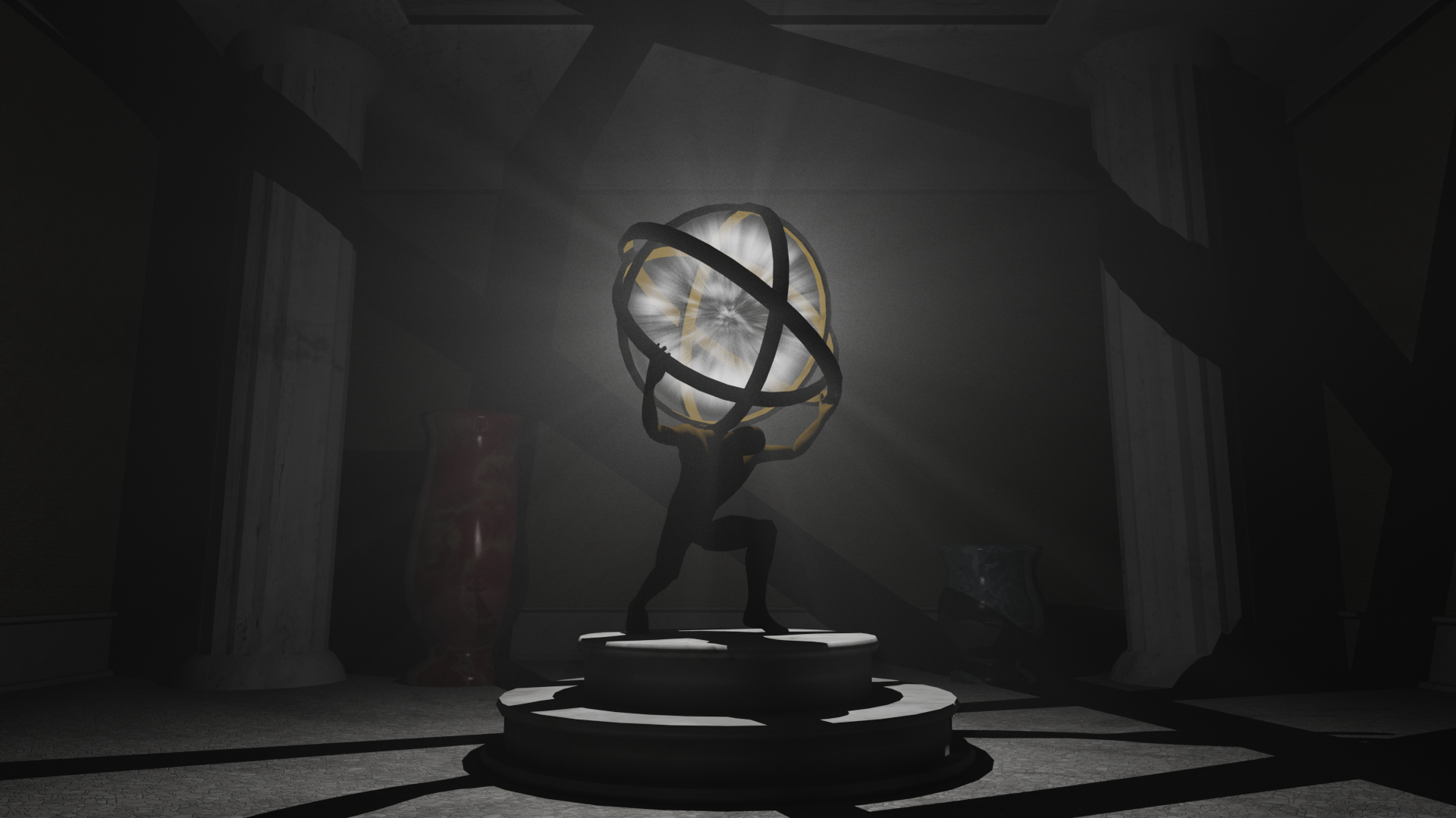
Final Scene.
Path Tracing
I implemented bidirectional path tracing.
For each sample two paths are generated: a camera path and a light path. The camera path starts with a camera ray, while the light path starts with a randomly selected light source and direction. The paths are built by repeatedly intersecting rays with the scene, recording the intersection point, and creating a new ray based on the material of the intersected primitive.
After both paths are generated, each camera vertex is connected to each light vertex to create many camera-light paths. The light throughput of each path \(P\) is calculated using the following equation:
\[P\left(\bar{s},\bar{t}\right) = C(s_n) f_{s_n}\left(s_{n-1},s_n,t_m\right) G\left(s_n,t_m\right) f_{t_m}\left(s_n,t_m,t_{m-1}\right) C(t_m) L(t_0) \]
Where \(\bar{s} = s_0\rightarrow s_1\rightarrow\cdots\rightarrow s_n\) is the camera path, \(\bar{t} = t_0\rightarrow t_1\rightarrow\cdots\rightarrow t_m\) is the light path, \(f_{s_n}\) and \(f_{t_m}\) are the surface BRDFs, \(L(t_0)\) is the direct light at the first light vertex, \(G(t_m,s)\) is an occlusion factor calculated by casting a shadow ray, and \(C(v)\) is the contribution of the vertex \(v\) and is calculated as the path is being constructed:
\[C(s_k) = \prod_{i=1}^{k-1} f_{s_{i}}(s_{i-1}\rightarrow s_{i} \rightarrow s_{i+1}) \]
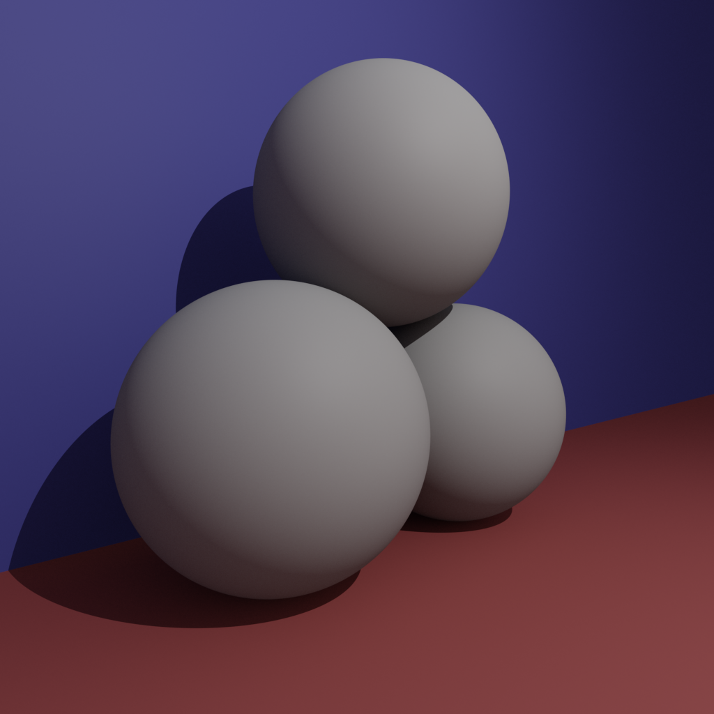
Notice the red floor colour bleeding onto the white spheres.
Soft Shadows
Soft shadows are a direct consequence of bidirectional path tracing and spherical light sources.
Spherical light sources are implemented by choosing a random point on the surface of the sphere and a random direction as the start of the light path.
This works well for scenes with only diffuse objects where the light itself is not visible; however, extra effort is done in order for camera rays to be able to intersect with the light directly, or for purely specular camera-light paths to be possible. To handle these cases, each spherical light source adds a sphere primitive to the scene with a special emissive material. When a camera path intersects with these emissive spheres, this emitted light is added to the output.
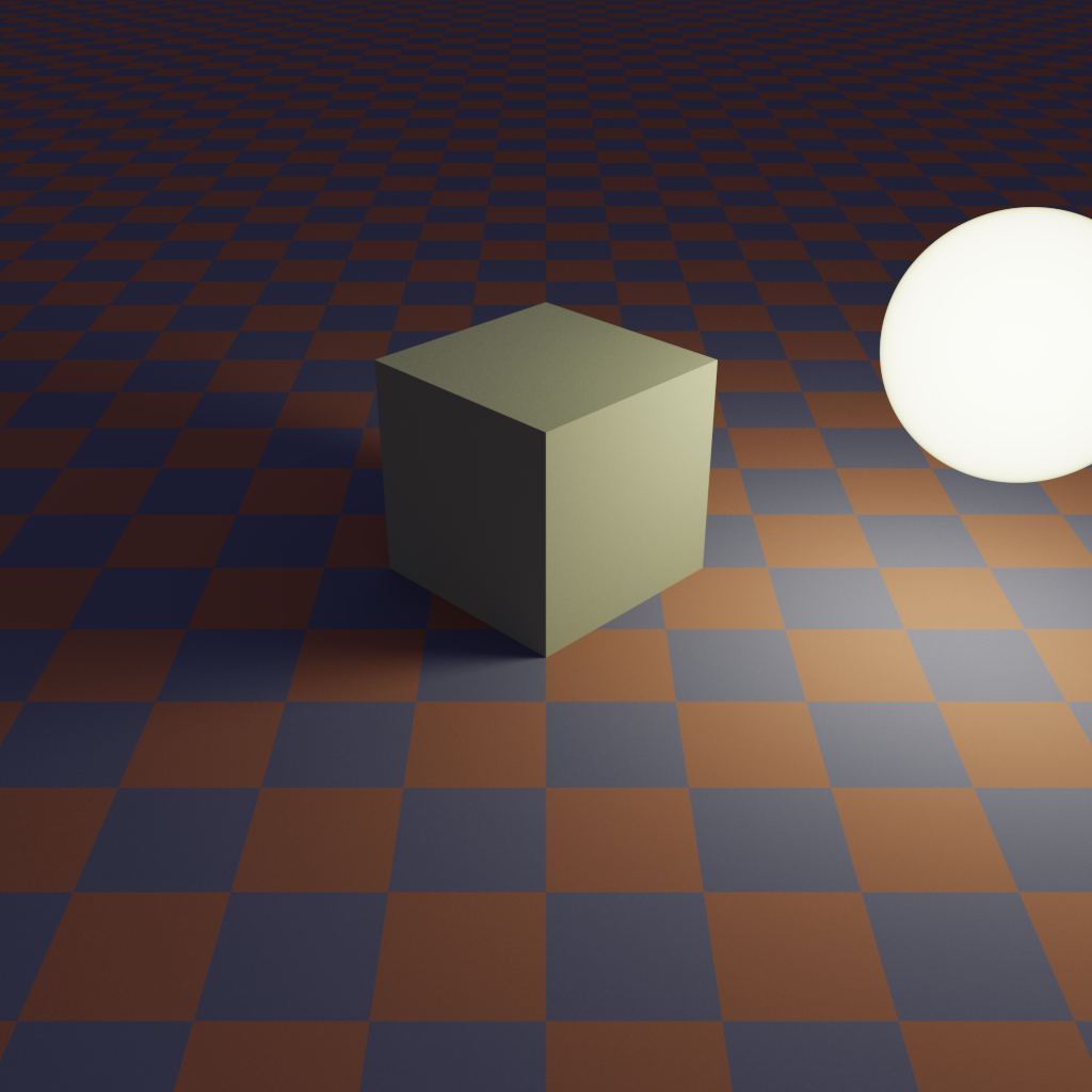
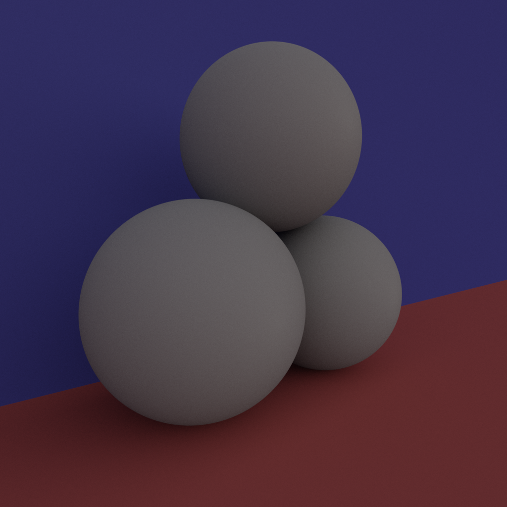
No direct light, uniform sky lighting only.
Point light and uniform sky lighting.
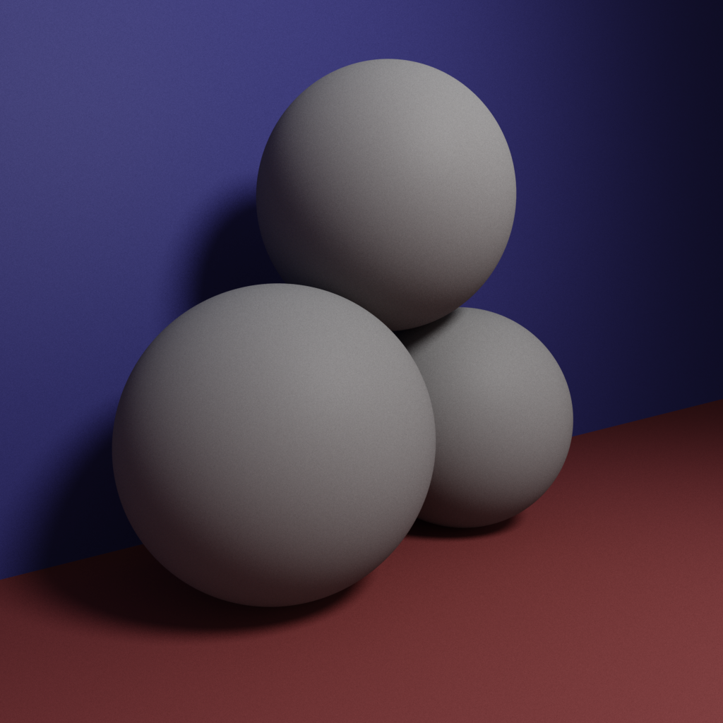
Spherical light and uniform sky lighting.
Refraction & Fresnel Effect
I implemented a glass-like material that has both reflection and refraction components combined together using the Fresnel equations.
In the following image, notice the reflections around the edges of the spheres and the caustic effects of the spheres on the floor.
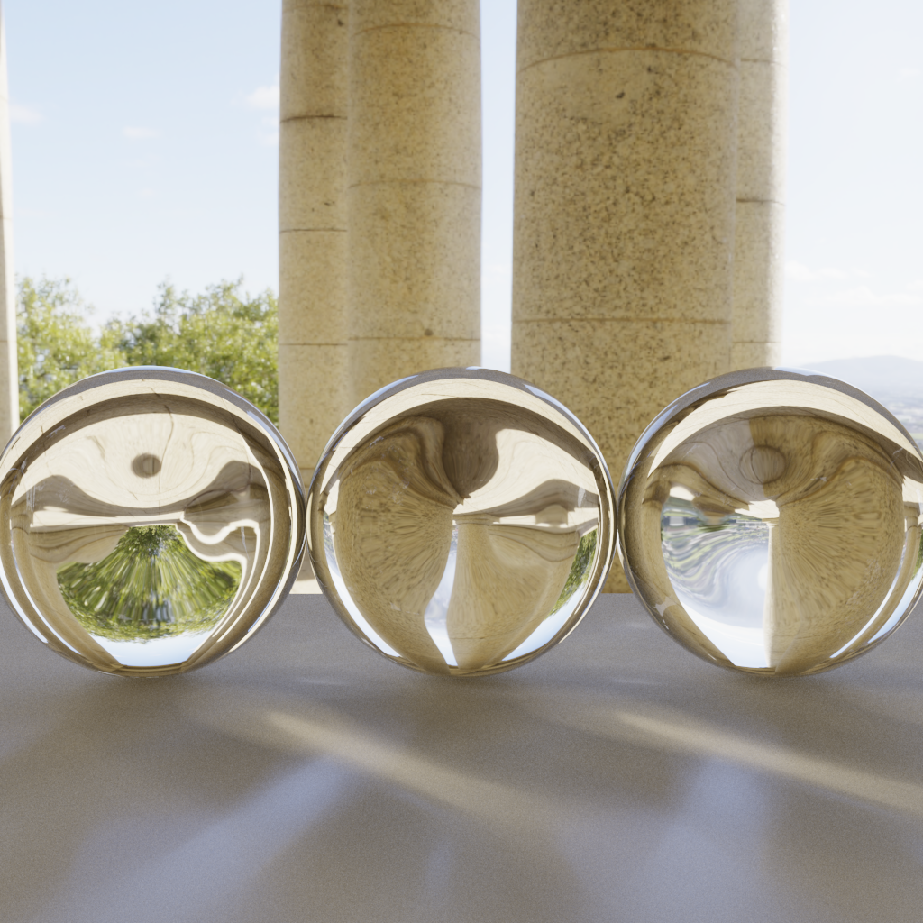
Glass spheres.
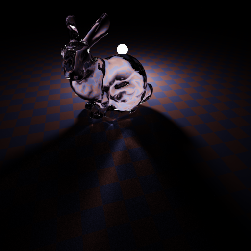
Stanford Bunny caustics.
Texture Mapping
I implemented texture mapping by storing the \(u\) and \(v\) coordinates of each intersection point and sampling textures once using linear interpolation. Antialiasing is achieved by simply taking more samples per pixel.
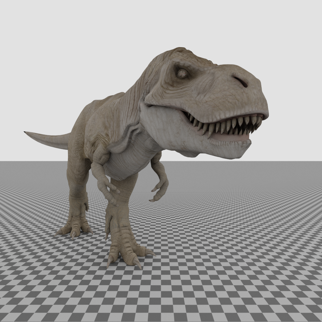
Textured T. rex and procedural checkerboard texture.
Bump Mapping
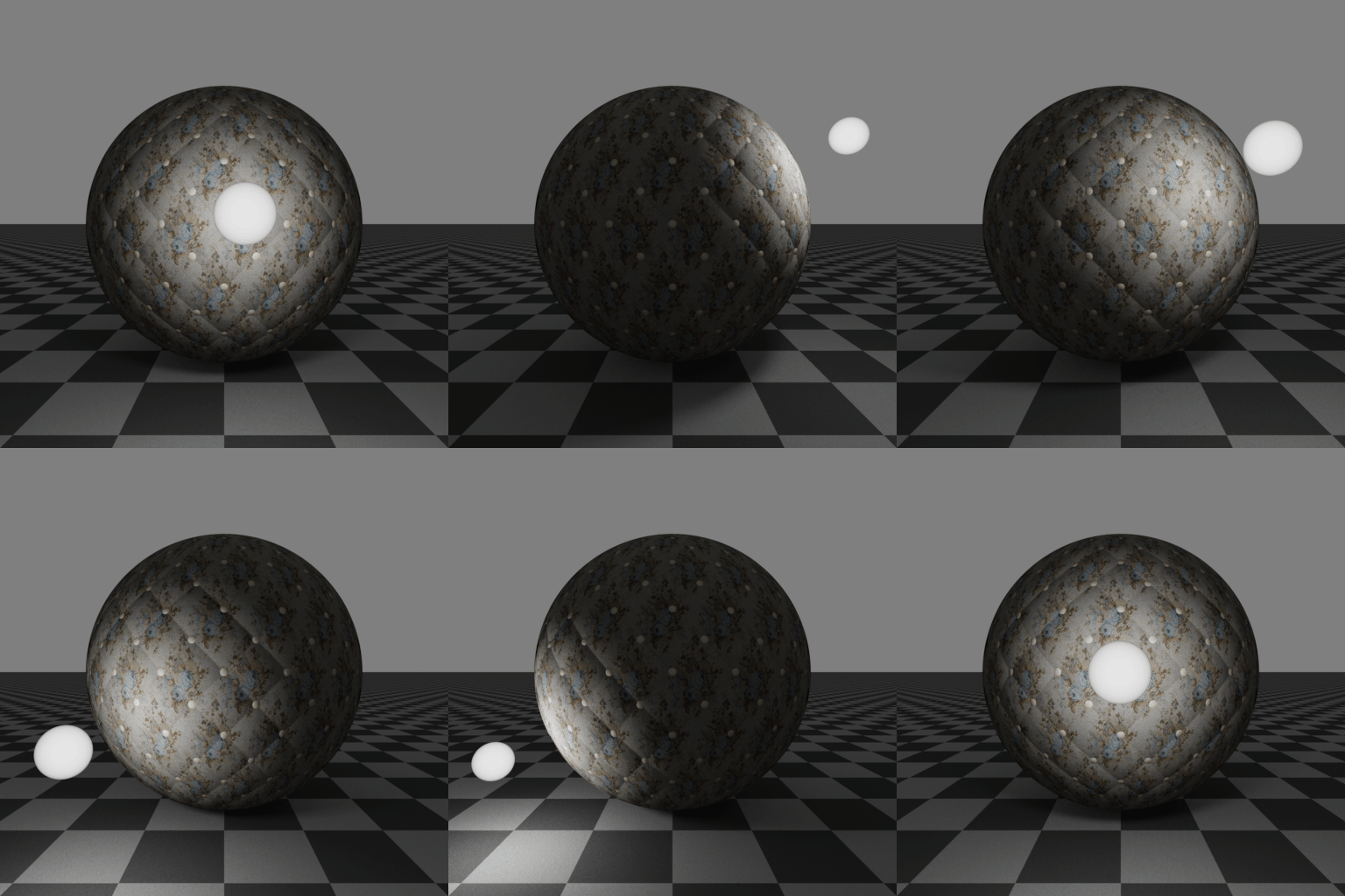
Bump mapping is implemented by storing the normal and \(u\) and \(v\) tangent vectors at each intersection point and perturbing the normal according to a sample from a normal map.
In the following animation, notice how the shading on the surface of the sphere changes as the light moves.
Perlin Noise
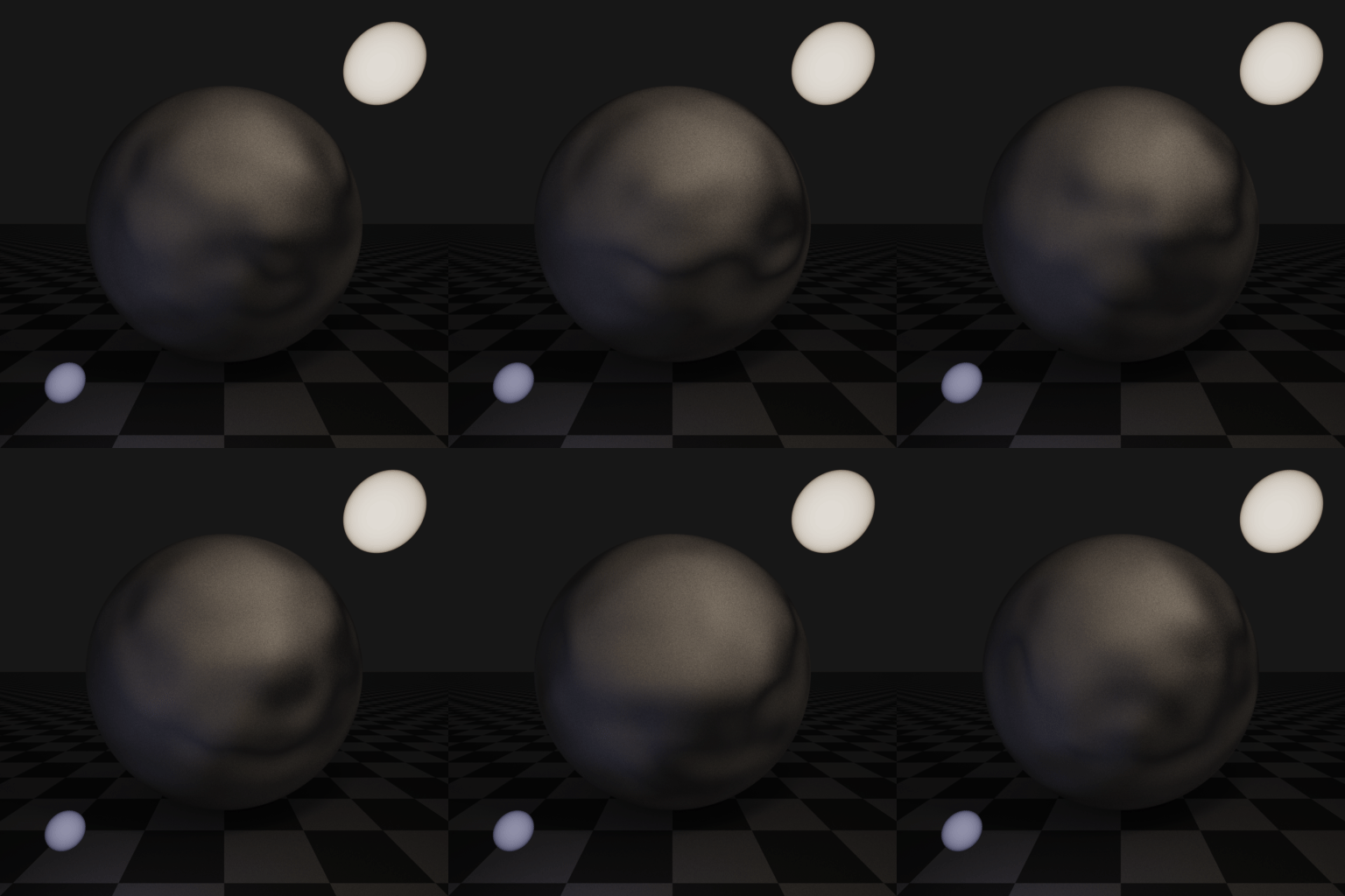
I implemented 3D and 4D Perlin noise using Perlin's improved interpolation technique.
The next animation is created by measuring the derivative of the Perlin noise at the surface of the sphere with respect to the \(u\) and \(v\) tangent vectors. These values are used to perturb the surface normal. I then create an animation using time as the fourth dimension of the Perlin noise input.
Depth of Field
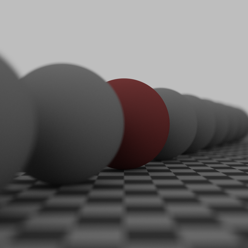
I implemented depth of field using the thin lens camera model. Each sample starts at a random point on the camera's aperture and is given a direction such that all rays for a specific pixel intersect at the same point on the focal plane.
Antialiasing
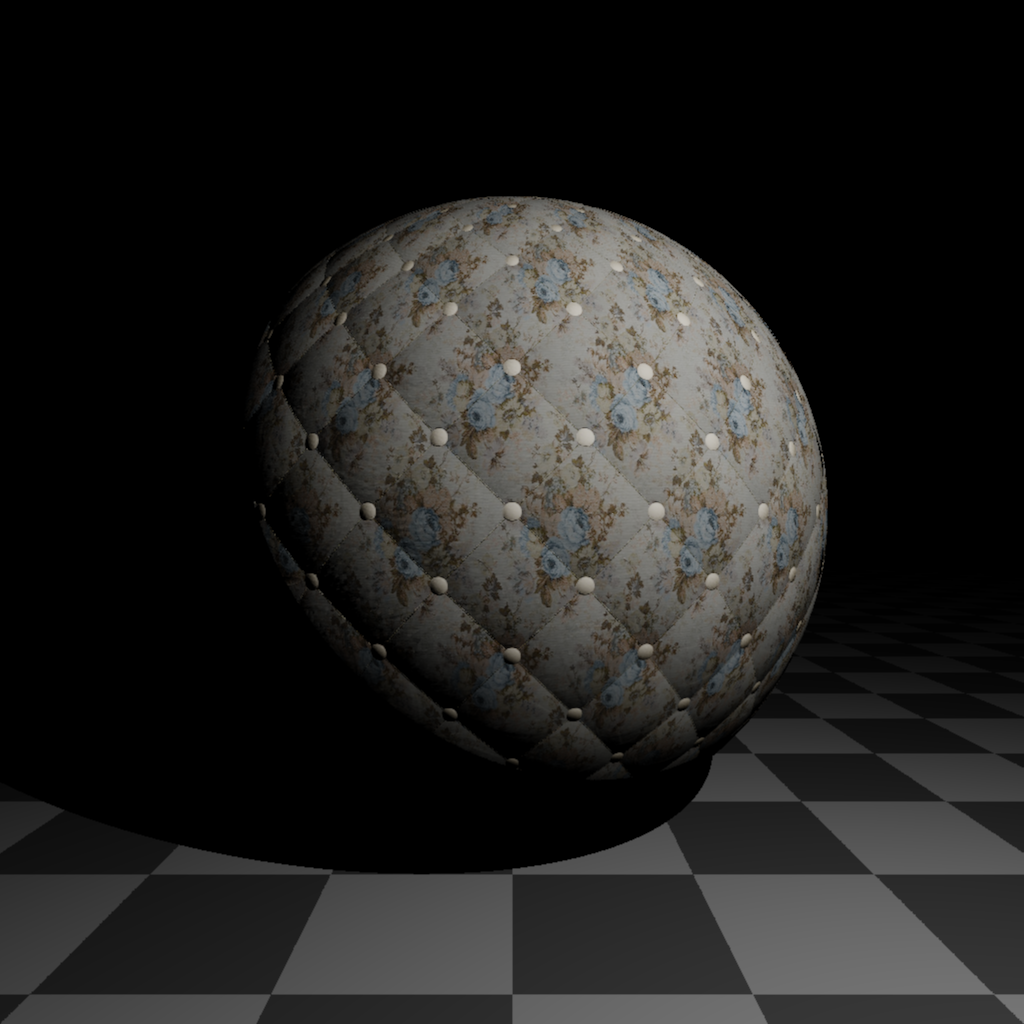
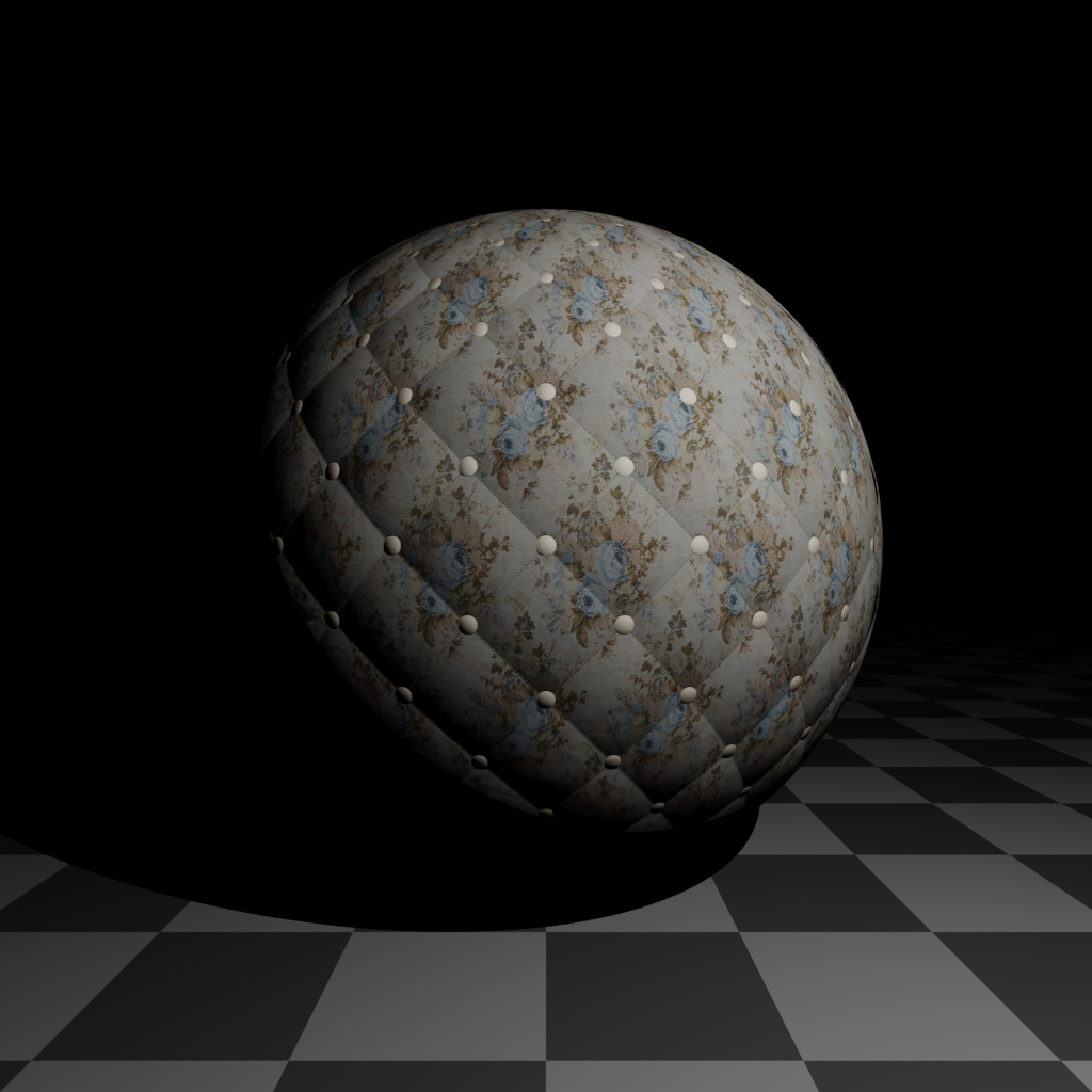
Multisample antialiasing is implemented by sampling rays not at the center of each pixel but at a uniformly random point within each pixel.
The first image is created by taking samples at the exact center of each pixel while the second is created by taking 8 samples randomly distributed within each pixel. In the first image, notice the jagged edges on the shadows and along the checkerboard lines. Those same lines are smooth in the second image.
Not antialiased.
Antialiased.
Acceleration
For acceleration, I implemented axis-aligned bounding box for each primitive and a k-d tree for storing the faces of each mesh. I also implemented multithreading by having each thread write to a thread-local buffer, accumulating all the buffers at the end.
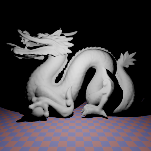
The following scene with the Stanford dragon model contains ~100,000 faces. In each test I rendered the scene at 512x512 resolution and with 8 samples per pixel.
I did the performance benchmarking on a 64 core Google Cloud Intel Skylake compute-optimized machine.
Without a mesh k-d tree and on a single thread it would take ~420 minutes to render the image. With a mesh k-d tree on a single thread it takes only 288 seconds -- An 87x improvement!.
The following charts show the multicore scaling with mesh k-d tree enabled. Up to 32 cores, the scaling is nearly perfect but drops off to 75% scaling at 64 cores. Using 64 cores and a k-d tree the scene can be rendered in just 5.95 seconds -- A 4000x improvement over no acceleration!
Opacity Mapping
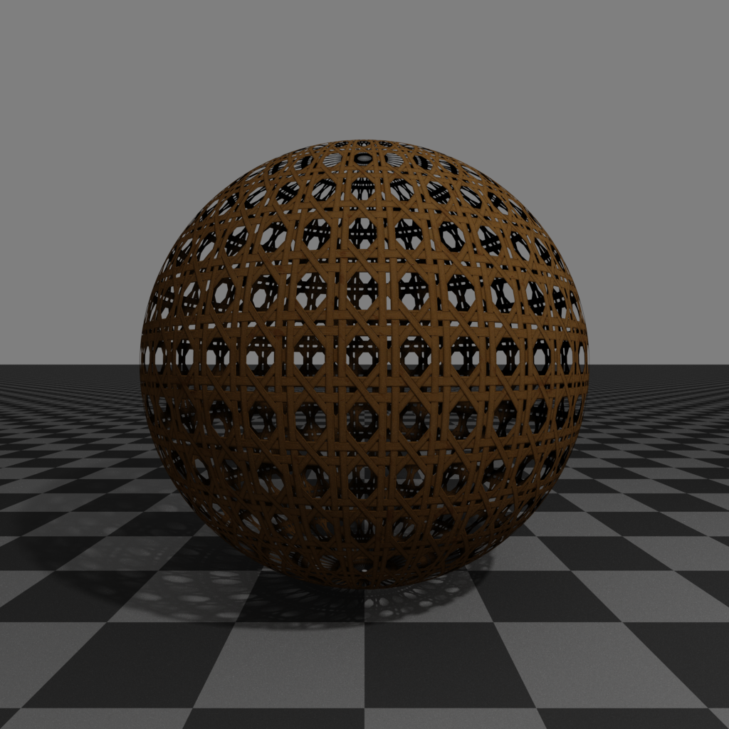
When constructing a path, if a ray intersects with a transparent part of a surface, the surface BRDF is ignored.
When a ray intersects with a transparent part of a surface during an occlusion test, that surface is ignored and a second ray is shot.
Glossy Reflections
I added glossy reflections to my material model by adding a reflectiveness parameter and a glossiness parameter. The reflectiveness parameter performs a linear interpolation between a Lambertian surface model and a perfect reflection model. The glossiness parameter that controls a random perturbation of the reflected ray and how sharp the BRDF is at the reflected angle.
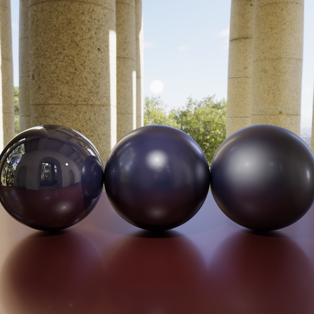
Three spheres with varying glossiness.
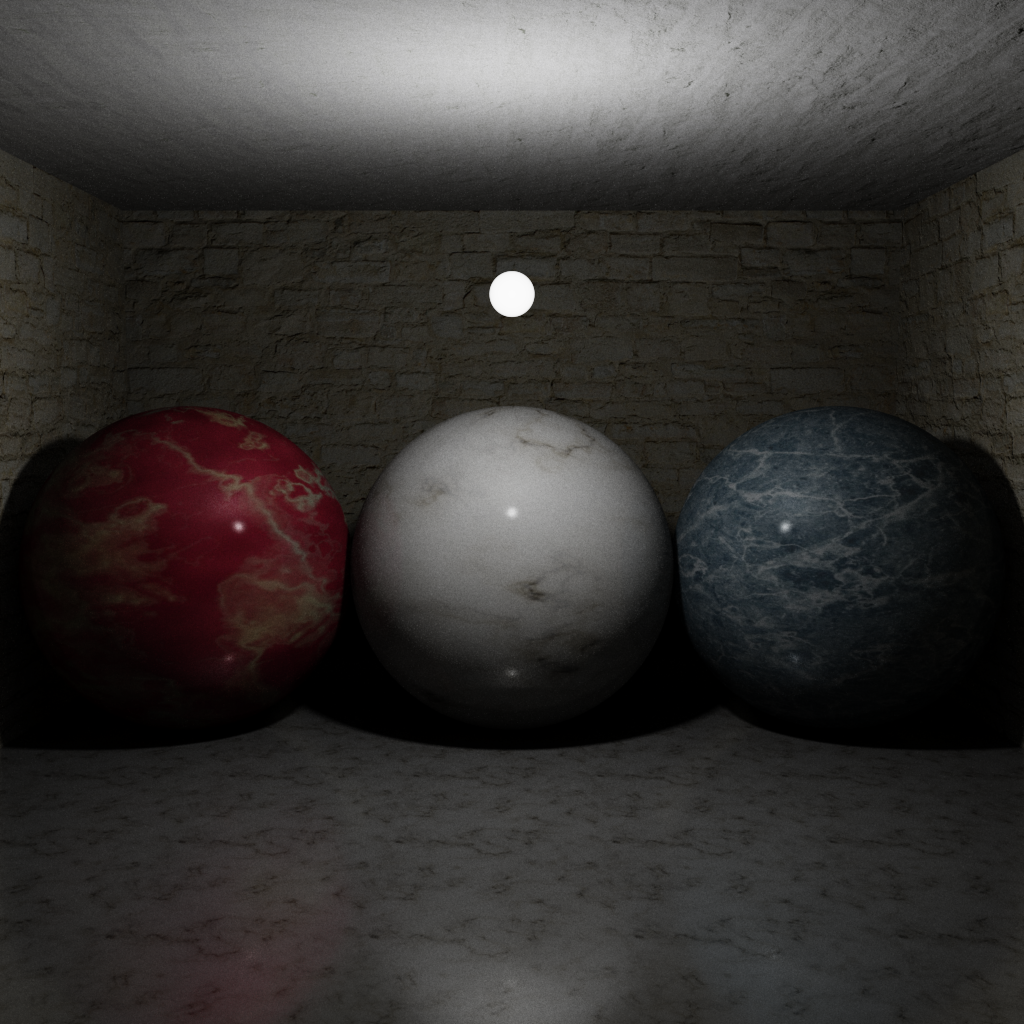
Textured materials with glossy reflections.
Metropolis Light Transport
I implemented pure sample space Metropolis light transport.
Each path is identified with the vector of random numbers used to generate it. By applying random mutations to this vector of numbers, a Markov chain of paths can be created. This Markov chain is then used as part of the Metropolis sampling algorithm to sample paths with probability density approximately equal to the luminance of the path.
I implemented two mutation types: a large step that completely randomizes the random vector and a small step that applies a small normally distributed perturbation to the vector.
This implementation still needs some tweaking to be usable and in general produces noisier results than standard bidirectional path tracing. To improve the results I would need to reduce startup bias by adopting a better approach for generating bootstrap samples. I could also implement a more sophisticated mutation strategy.
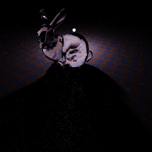
Standard BDPT, 32 Samples.
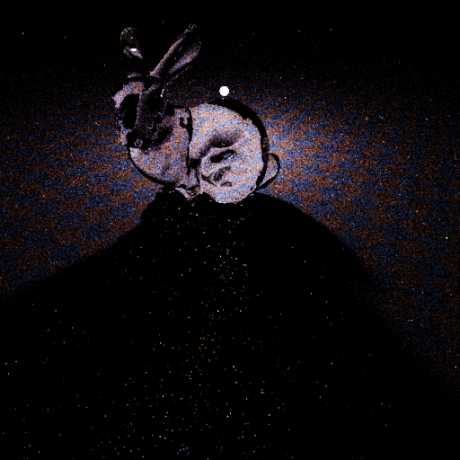
Metropolis Light Transport, 32 Samples.
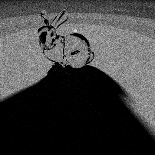
Metropolis Light Transport samples per pixel.
Volumetric Scattering
I implemented volumetric scattering by assigning each object in the scene an internal medium and also designating a global scene medium.
As paths are being constructed, I keep track of the medium that the current ray is travelling through. Before adding a vertex to the path, I first consider the possibility that the light will scatter before reaching the intersection point. In this case a special scattering vertex is added to the path instead of the usual intersection vertex.To calculating the throughput of each path, the equation described above is modified to:
\[P\left(\bar{s},\bar{t}\right) = C(s_n) f_{s_n}\left(s_{n-1},s_n,t_m\right) T\left(s_n,t_m\right) f_{t_m}\left(s_n,t_m,t_{m-1}\right) C(t_m) L(t_0) \]
Where the occlusion factor \(G(s_n, t_m)\) has been replaced by a transmittance factor \(T(s_n, t_m)\), \(f_{s_n}\) and \(f_{t_m}\) are either surface BRDFs or scattering phase functions, and \(C(v)\) has been modified to
\[C(s_k) = T(s_0,s_1)\prod_{i=1}^{k-1} (f_{s_{i}}(s_{i-1}\rightarrow s_{i} \rightarrow s_{i+1})T(s_{i-1},s_{i}))T(s_{k-1},s_k) \]
Light scattering in a homogeneous medium ray is a Poisson process so the scattering distance follows an exponential distribution. Given a value \(x\) generated from a uniform random distribution the exact scattering distance is calculated using the inverse CDF:
\[\frac{-\text{log}(1-x)}{\sigma}\]
Where \(\sigma\) is the number of scattering events per unit distance.
To calculate the transmittance between two points in a homogeneous medium, the CDF of the complement of the scattering event is used:
\[ T(s_n,t_m) = e^{-\sigma \|s_n - t_m\|} \]
For non-homogeneous mediums, I used ray marching, where the inverse CDF is approximated by integrating the PDF by sampling at fixed intervals.
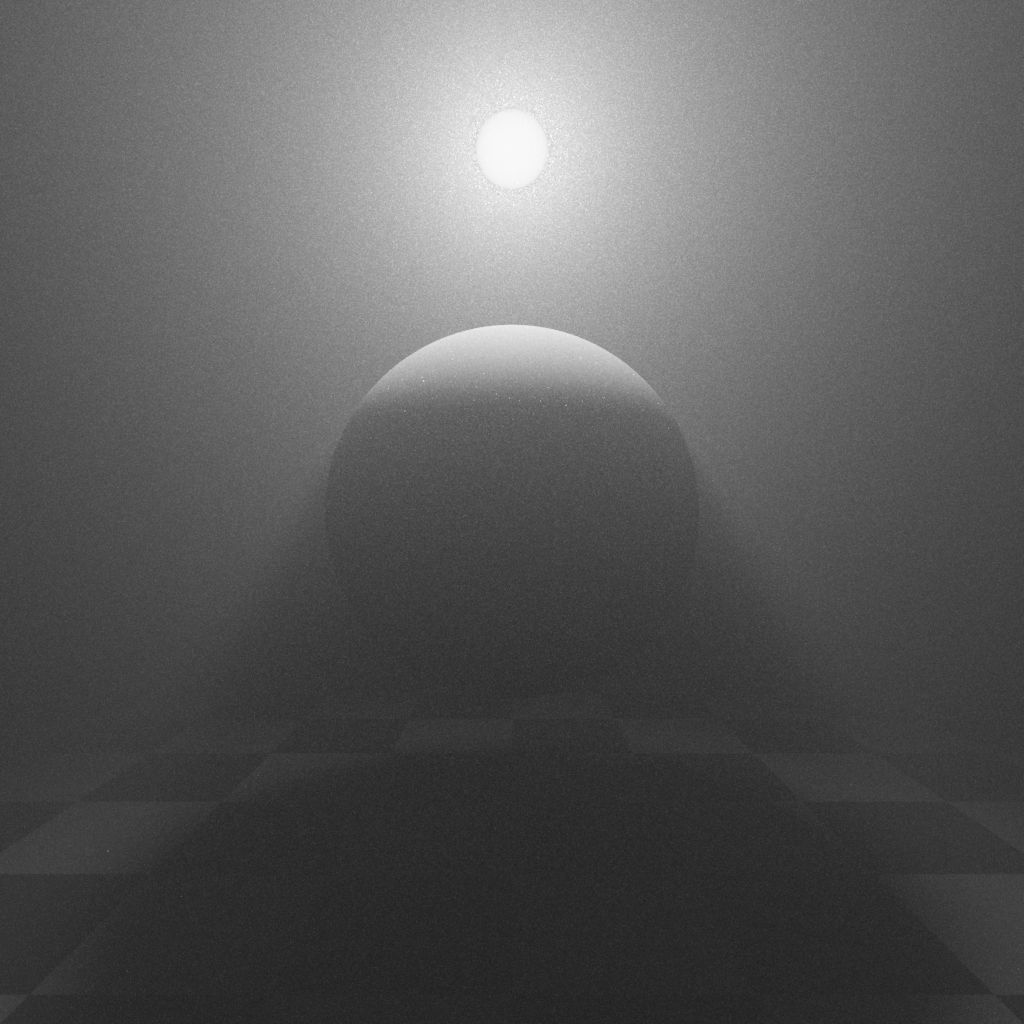
Homogeneous global medium.
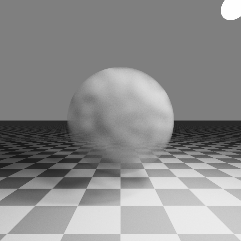
Medium contained within a sphere using ray marching over Perlin noise.
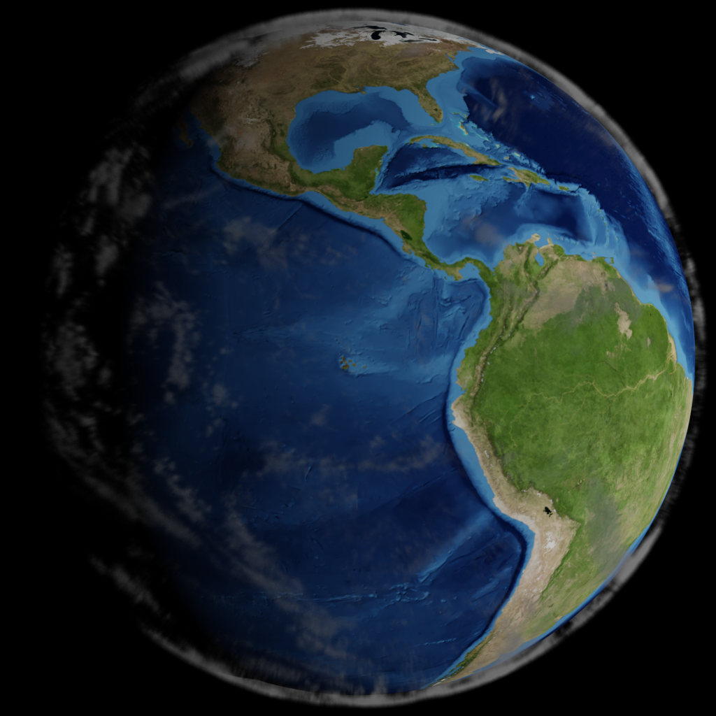
Clouds rendered using ray marching on NASA's blue marble imagery.
Final Scene
My final scene is inspired by Greek Mythology. After the war of the Titans, Zeus condemns the Titan Atlas to hold up the sky. This is my interpretation of that myth.
To render the "sky", I used a distorted version of the ray-marching medium using NASA's "Blue Marble" imagery. The god-ray effect is caused by the rings of the statue casting shadows through a homogeneous global medium.
The final scene is rendered at 1920x1080 with 2048 samples per pixel. It took ~11 hours to render on a 64 core Google cloud compute machine.
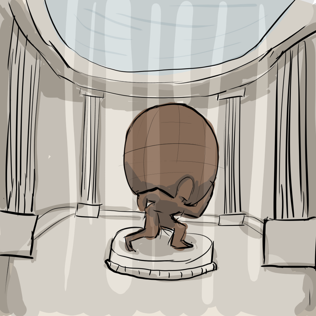
Final scene concept sketch.
Final Scene.
Credits
Credit to Greg Zaal and hdrihaven.com for the hdri skyboxes used in some of the renders above.
Credit to joel3d at turbosquid.com for the T. rex model used in the texture mapping render.
Credit to CG_Luke at turbosquid.com for the human base model used in the final scene.
Credit to the Stanford 3D Scanning Repository for the Stanford Bunny and Stanford Dragon models.
Credit to NASA for the Blue Marble imagery.
Credit to 3dtextures.me for the rest of the textures used.
Credit to Bruce Walter for his implementation of the RGBE file format.
I used the sol library for extending the lua interface.